Oscilloscope
You will be surprised that the EV3 text display can be tweaked to create an oscilloscope.
The EV3 display
The EV3 has a 178 × 128 pixel Monochrome display. The corners have these coordinates:
- top-left - (1, 1)
- bottom-left - (1, 128)
- top-right - (178, 1)
- buttom-right - (178, 128)
It can display:
- 12.8 lines of small text
- 22 characters long
The small character occupy 10x8 pixels. One character is
- 9 pixels high
- 7 pixels wide
For exemple an A is composed of these pixels:
1 2 3 4 5 6 7
      x
      x
    x   x
    x   x
  x       x
  x       x
  x x x x x
x           x
x           x
Characters used
For the oscilloscope we are going to use the vertical bar:
1 2 3 4 5 6 7
      x
      x
      x
      x
      x
      x
      x
      x
      x
the horizontal bar (underscore):
1 2 3 4 5 6 7

x x x x x x x
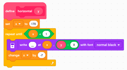
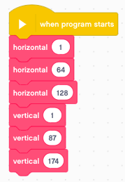
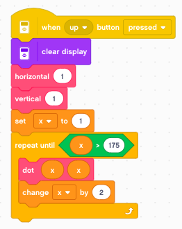
Display a horizontal line
With this information we are ready to display a horizontal line at position y. We define the variables x and y.
We write backwards. The reason for this is that the 7x9 pixel character is printed on a 8x10 pixel field. In fact the left and the top 1-pixel-wide line is erased.
So we initialize x to 178, and decrement by the caracter width of 7. With regards to y there is a -8 pixel offset.
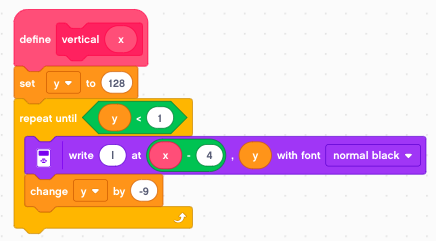
Display a vertical line
Then we define the vertical(x) function.
So we initialize y to 128, and decrement by the caracter height of 9. With regards to x there is a -4 pixel offset.
Draw a dot
The function write text at (x, y) can place a character at the position (x, y).
To draw an arbitrary curve using dots, we could use the dot (.) or the hyphen (-).
But the best way is to use an underscore (_) followed by a space character.
The space character is offset by 2 pixels and erases the 6 unused pixels of the underscore.
This allows us to draw a dot every 2nd pixel.
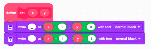
The example below draws a diagonal line starting at (1, 1).
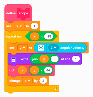
Display a scope trace
Now we have all the elements to program an oscilloscope. We start at x=1 and loop until x>175. At each iteration we increase x by 2.
The y value is the angular gyro velocity. We display it numerically on line 1. And we plot it with an offset of 64 to the screen.
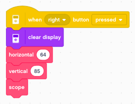
With a button press we can acquire a single trace of 88 samples.
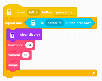
Measure continously
We can place it inside a loop and measure continously.
You can download the programs so far:
scope.lmsp